Normal vs. Lognormal Volatility

There are two common methods for measuring volatility: normal volatility and lognormal volatility.

Visit the Mammoth Options Pricing System, supporting FX options and structured products pricing and valuation!

I. Introduction: Origins and Significance of the Two Volatility Paradigms

In the field of financial derivatives pricing and risk management, the way volatility is characterized fundamentally determines the behavior of models. Historically, two main paradigms for describing volatility have developed in parallel:

1. Normal (Bachelier) Volatility: Proposed by Louis Bachelier in 1900, it measures the standard deviation of absolute price changes and applies to arithmetic Brownian motion.
2. Lognormal (Black-Scholes) Volatility: Refined by Black, Scholes, and Merton in 1973, it is based on the standard deviation of logarithmic returns, corresponding to geometric Brownian motion.

These seemingly simple differences lead to profound distinctions in mathematical properties, market applicability, and risk management. This article systematically analyzes their theoretical foundations, calculation methods, conversion relationships, and practical applications.

II. Mathematical Essence and Core Formulas

1. Normal Volatility (σₙ)

Definition: Annualized standard deviation of absolute price changes
Stochastic Process:

$$dS_t = \sigma_n dW_t$$

Discrete Form:

$$S_{t+\Delta t} = S_t + \sigma_n \sqrt{\Delta t} Z, \quad Z \sim N(0,1)$$

Properties:

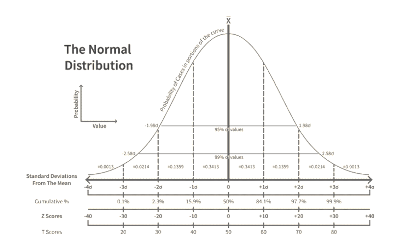
• Price changes ΔS follow a normal distribution$N(0, \sigma_n^2 \Delta t)$.
• Negative prices are allowed.
• Volatility units match price units (e.g., USD/year).

image-20250617100754507

2. Lognormal Volatility (σₗₙ)

Definition: Annualized standard deviation of logarithmic returns
Stochastic Process:

$$d\ln S_t = \left(\mu - \frac{1}{2}\sigma_{ln}^2\right)dt + \sigma_{ln} dW_t$$

Discrete Form:

$$S_{t+\Delta t} = S_t \exp\left[\left(\mu - \frac{1}{2}\sigma_{ln}^2\right)\Delta t + \sigma_{ln} \sqrt{\Delta t} Z\right]$$

Properties:

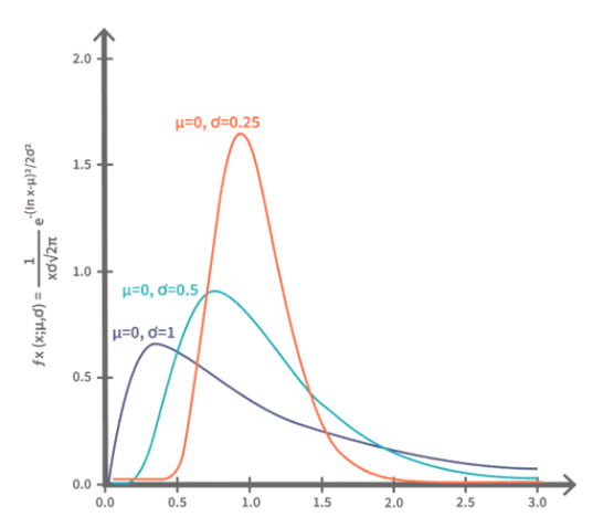
• Logarithmic returns$\ln(S_t/S_0)$follow a normal distribution.
• Prices are strictly positive.
• Volatility units are percentages (e.g., 20%/year).

image-20250617100805668

3. Conversion Relationship

For short-term/small volatility conditions:

$$\sigma_n \approx S_0 \times \sigma_{ln}$$

For precise conversion, convexity adjustment is required:

$$\sigma_n = S_0 \sigma_{ln} \sqrt{T} \left(1 + \frac{1}{2}\sigma_{ln}^2 T \right)$$

4. Brownian Motion and Its Relationship with the Two Models

1. Mathematical Basis of Brownian Motion

Brownian Motion (also known as Wiener Process) is the core stochastic process underlying both models, defined as:

$$W_t \sim N(0, t)$$

Properties:

• Independent increments:$W_{t+\Delta t} - W_t$is independent of historical paths.
• Normal distribution:$\Delta W_t \sim N(0, \Delta t)$.
• Continuous but non-differentiable paths.

2. Application in the Bachelier Model

The normal model directly uses the additive property of Brownian Motion:

$$dS_t = \sigma_n dW_t$$

• Economic Interpretation: Price changes$\Delta S_t$are linear scalings of Brownian Motion increments.
• Discrete Form:

$$S_{t+\Delta t} = S_t + \sigma_n \Delta W_t$$

• Distribution Characteristics: Prices follow$N(S_0, \sigma_n^2 t)$, preserving the possibility of negative values.

Example:
If$\sigma_n = 20$bps/√year, the standard deviation of price changes after one day:

$$\sigma_n \sqrt{1/252} = 20 \times 0.063 \approx 1.26 \text{bps}$$

3. Transformation in the Black-Scholes Model

The lognormal model introduces multiplicative noise via logarithmic transformation:

$$d\ln S_t = \left(\mu - \frac{1}{2}\sigma_{ln}^2\right)dt + \sigma_{ln} dW_t$$

• Economic Interpretation: Returns$d\ln S_t$combine drift terms with Brownian Motion.
• Discrete Form:

$$S_{t+\Delta t} = S_t \exp\left[(\mu-\frac{1}{2}\sigma_{ln}^2)\Delta t + \sigma_{ln} \Delta W_t\right]$$

• Distribution Characteristics: Logarithmic prices follow a normal distribution, ensuring$S_t > 0$.

Example:
If$\sigma_{ln} = 20\%$, the standard deviation of returns after one day:

$$\sigma_{ln} \sqrt{1/252} \approx 1.26\%$$

III. Comparison of Simple Option Pricing Formulas

1. Call Option Pricing

Bachelier (Normal) Model:

$$C = (S_0 - K)\Phi(d) + \sigma_n \sqrt{T} \phi(d)$$

$$d = \frac{S_0 - K}{\sigma_n \sqrt{T}}$$

Black-Scholes (Lognormal) Model:

$$C = S_0 \Phi(d_1) - K e^{-rT} \Phi(d_2)$$

$$d_1 = \frac{\ln(S_0/K) + (r + \sigma_{ln}^2/2)T}{\sigma_{ln} \sqrt{T}}$$

$$d_2 = d_1 - \sigma_{ln} \sqrt{T}$$

Example Calculation (S₀=100, K=105, T=1, r=0):

• Normal: σₙ=20 USD → C≈7.12
• Lognormal: σₗₙ=20% → C≈6.89

2. Put Option Pricing

Bachelier Model:

$$P = (K - S_0)\Phi(-d) + \sigma_n \sqrt{T} \phi(d)$$

Black-Scholes Model:

$$P = K e^{-rT} \Phi(-d_2) - S_0 \Phi(-d_1)$$

IV. Market Quotation Examples

1. FX Market (Lognormal Convention)

Quotation Characteristics:

• Implied volatility quoted under the Black-Scholes model.
• Volatility surface uses Delta as the horizontal axis.
• Standard format example:

Tenor	ATM	25D RR	25D BF
1M	11.2%	-0.5%	0.7%
1Y	10.5%	-1.2%	1.0%

Where:

• ATM: At-the-money volatility.
• RR (Risk Reversal): Call-Put volatility spread.
• BF (Butterfly): Volatility convexity adjustment.

2. Interest Rate Market (Normal Convention)

Cap/Floor Quotations:

• Volatility typically quoted under the Bachelier model.
• In basis points (bps).
• Market data example:

image-20250617093449078

(1) Column Definitions

Column Name	Description
Period	Option tenor (1Y=1 year, 30Y=30 years, etc.)
Strike	Strike price of ATM option (in %, e.g., -0.340%=negative rates scenario)
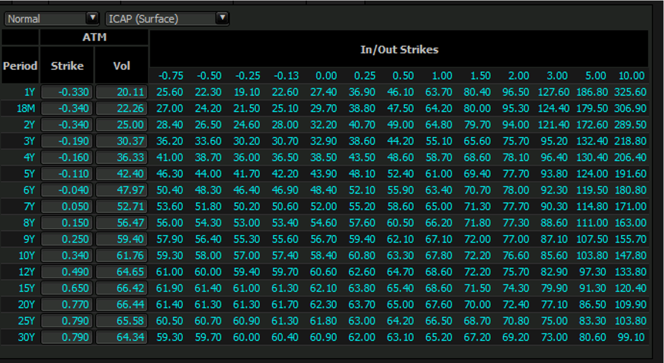
Vol	Normal volatility of ATM option (in bps)
In/Out Strikes	Volatility quotes for different strikes (in bps), with strike intervals in %.

(2) Example Analysis (1Y Tenor)

Strike	-0.75%	-0.50%	...	10.00%
Vol	27.00	24.20	...	306.90

• Economic Meaning:
  For a 1-year cap option with a strike of -0.75%, the market quotes a volatility of 27 bps (i.e., the annualized standard deviation of expected absolute rate changes is 0.27%).

Why Normal Volatility?

Interest rate markets use the Bachelier model (normal volatility) due to:

1. Negative Rate Possibility: Negative strikes (e.g., -0.33%) cannot be handled by the lognormal model.
2. Linear Sensitivity: DV01 (price change per 1bp rate move) aligns better with normal assumptions.
3. Market Convention: Global interest rate options (e.g., Caps/Floors, Swaptions) typically quote volatility in bps.

V. Practical Volatility Conversion

FX Option Conversion Example

Given:

• EUR/USD spot = 1.1000
• 1Y ATM implied volatility = 12% (lognormal)
• Convert to normal volatility.

Calculation:

$$\sigma_n \approx 1.1000 \times 12\% = 0.132 \text{ (132 pips)}$$

Precise Conversion (T=1):

$$\sigma_n = 1.1000 \times 12\% \times (1 + \frac{1}{2}0.12^2 \times 1) = 0.139 \text{ (139 pips)}$$

Interest Rate Cap Conversion Example

Given:

• 3M LIBOR forward = 2.5%
• Normal volatility = 50 bps
• Convert to lognormal volatility.

Calculation:

$$\sigma_{ln} \approx \frac{50 \text{bps}}{2.5\%} = 20\%$$

Precise Conversion:

$$\sigma_{ln} = \frac{50 \text{bps}}{2.5\%} \left(1 - \frac{(50 \text{bps})^2 \times 1}{2 \times (2.5\%)^2}\right) \approx 18.5\%$$

VI. Price Vol vs. Yield Vol: Key Relationships

Price Vol (price volatility) and Yield Vol (yield volatility) are two ways to measure asset price or yield fluctuations in financial markets. Their core differences lie in units of measurement and applicability, but they can be converted mathematically. Below is a detailed comparison and analysis of their relationship.

1. Definitions and Core Differences

Type	Price Vol (Price Volatility)	Yield Vol (Yield Volatility)
Definition	Standard deviation of absolute price changes (e.g., USD, bps)	Standard deviation of percentage price changes (returns) (e.g., 20%)
Units	Same as price (e.g.,$5/year, 50 bps)	Percentage (e.g., 20%)
Model	Bachelier (Normal Model)	Black-Scholes (Lognormal Model)
Typical Markets	Interest rate derivatives (Caps/Floors), commodity options	Equities, FX, bond yield options
Negative Values?	Yes (e.g., negative rates)	No (logarithmic transformation ensures positivity)

2. Mathematical Relationship

(1) Short-Term Approximation

For short-term or low-volatility scenarios, Price Vol (σₙ) and Yield Vol (σₗₙ) can be approximated as:

$$\sigma_n \approx S_0 \times \sigma_{ln}$$

Examples:

• Stock price =$100, Yield Vol = 20% →

$$\text{Price Vol} \approx 100 \times 0.20 = \$20/\text{year}$$

• Bond yield = 2%, Yield Vol = 10% →

$$\text{Price Vol} \approx 2\% \times 0.10 = 0.2\% \text{ (20 bps)}$$

(2) Precise Conversion (Convexity Adjustment)

For long-term or high-volatility scenarios, adjustments are needed:

$$\sigma_n = S_0 \sigma_{ln} \sqrt{T} \left(1 + \frac{1}{2} \sigma_{ln}^2 T \right)$$

$$\sigma_{ln} = \frac{\sigma_n}{S_0} \left(1 - \frac{\sigma_n^2 T}{2 S_0^2} \right)$$

Example:

• Stock price =$100, Yield Vol = 30%, T = 1 year →

$$\sigma_n = 100 \times 0.30 \times \left(1 + \frac{0.3^2 \times 1}{2}\right) = 31.5 \text{ USD/year}$$

3. Market Quotation Examples

(1) Interest Rate Market (Price Vol Dominant)

• Product: Interest rate cap.
• Quotation: 50 bps (standard deviation of absolute rate changes = 0.50%).
• Conversion: If current rate = 2%, equivalent Yield Vol ≈ 50 bps / 2% = 25%.

(2) Equity Market (Yield Vol Dominant)

• Product: Equity options.
• Quotation: 30% (annualized standard deviation of stock returns = 30%).
• Conversion: If stock price =$100, equivalent Price Vol ≈$30/year.

VII. Market Conventions Summary

Market Type	Default Volatility Type	Typical Quotation	Major Products
FX	Lognormal, Yield Vol	Percentage (e.g., 12%)	EUR/USD options
Interest Rates	Normal, Price Vol	Basis points (e.g., 50bps)	LIBOR caps/floors
Equities	Lognormal, Yield Vol	Percentage (e.g., 30%)	SPX options
Commodities	Hybrid	Both	Crude oil options